
















This post has been authored by Karel Bartos and Martin Rehak
The volume of the network traffic has been steadily increasing in the last years. In the same time, the delivery of critical services from cloud data centers has increased not only the volume of traffic, but also the complexity of transactions.
High volumes of network traffic allow the attackers to effectively hide their presence in the background. Moreover, attackers can shift or deceive the internal models of detection systems by creating large bursts of non-malicious network activity. Such activity typically draws an attention of statistical detection methods and is further reported as anomalous incident, while the important, yet much smaller malicious activity would remain unrecognized. To counter this, we need to deploy more sophisticated detection models and algorithms to detect such small and hidden attacks. The increase in volume of the transaction logs also brings computational problems for such algorithms, as they may easily become increasingly difficult to compute on the full traffic log.
Sampling reduces the amount of input network data that is further analyzed by the detection system, allowing the system of arbitrary complexity to operate on network links regardless of their size. However, the use of sampled data for CTA would be problematic, as it negatively impacts the efficacy. CTA algorithms are based on statistical traffic analysis and adaptive pattern recognition, and the distortion of traffic features can significantly increase the error rate of these underlying methods by breaking their assumptions about the traffic characteristics. The loss of information introduced by sampling methods also negatively impacts any forensics investigation.
First, let's have a look at an example of unsampled traffic in one dimension. For these examples, we are focusing on the number of flows originating from each source IP address. The corresponding feature distribution for 20 source IP addresses is illustrated in Figure 1. Since the feature values are computed from the original (unsampled) input data, there is no loss of information and the distribution is not biased. This is the ideal case. Unfortunately, as we mentioned earlier, the computational demands of more sophisticated algorithms require reducing the input data to be able to complete the processing in the given timeframe. So we need to apply sampling and we want to get sampling results as close to this distribution as possible

Figure 1. Number of flows for 20 source IP addresses computed from the original (unsampled) data. The distribution is unbiased, however the computational demands of the detection algorithms are high.
In the next three examples, we will reduce the size of input data to manage the cost of detection. First, we will try random sampling (either packet or flow-based), which is widely used thanks to its simple implementation and low computational demands. This sampling first randomly selects packets or flows and then computes features and performs detection. We will denote this sampling asearly random sampling. It has been proven that early random sampling negatively impacts the efficacy of most detection or classification methods. An example of such impact is illustrated in Figure 2. In contrast to the original distribution (Figure 1), early random sampling does not only affect the shape of the distribution, but also eliminates most of the rare feature values. You can see that this sampling completely eliminated all flows from 8 source IP addresses (IP2, IP13, IP15-IP20) and the remaining feature values are not precise. Most importantly, the eliminated values are typically the ones that should be discovered and reported as potentially malicious.
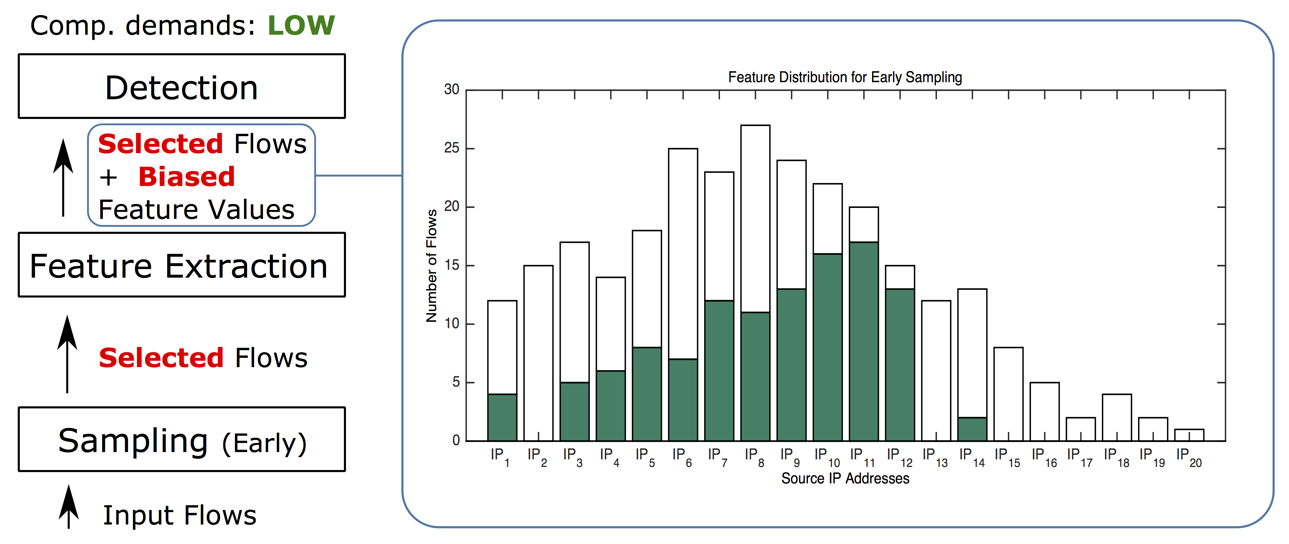
Figure 2. The effect ofearly randomsampling on feature distribution. Due to the fact that the flows are first randomly selected and the feature values are computed afterwards, early random sampling negatively shifted the feature distribution. You can see that flows originated from 8 source IP addresses were eliminated completely (pure white bars), while the rest of the values are highly imprecise.
In the next example, we dedicated some computational power to extract feature values from the original (unsampled) data before the sampling. This guarantees that our feature values are not biased. Once the feature values are computed, random sampling reduces the number of input flows for the detection algorithms. We call this methodlate random sampling. Figure 3 illustrates the resulting effect on our feature distribution. Bias introduced by the early sampling is significantly reduced, which rapidly improves the detection performance of statistical methods. However, flows from eight source IP addresses are still missing as none of them was selected by the random sampling.
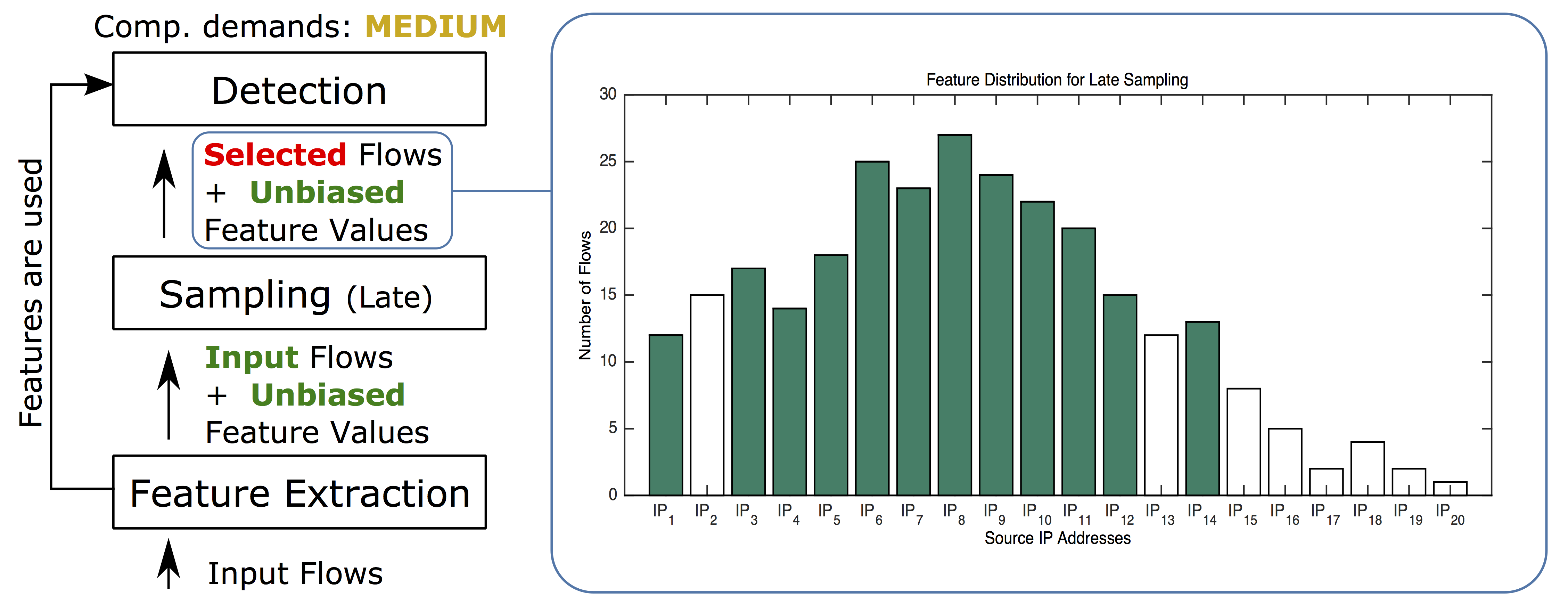
Figure 3.Late randomsampling preserves unbiased feature values of flows that are selected by sampling. However, source IP addresses with small number of flows are still eliminated.
In the last example, we presentlate adaptive sampling. It improves on late sampling by modification the sampling rate of flows according to their feature values to maximize the variability of the surviving samples. The late adaptive sampling selects flows according to the size of their feature values in order to de-emphasize large, visible and easily detectable events, and to select rare events (often related to hidden malicious activity) more frequently. The combination of adaptive and late sampling minimizes the bias of feature distributions important for the consequent detection methods, as illustrated in Figure 4.Late sampling allows the adaptive sampling to emphasize the conservation of the variability in the data, as the proportions have been conserved by feature extraction.

Figure 4. Adaptivesampling increases the variability of flows (and the number of source IP addresses) selected to the sampled set, whilelatesampling preserves unbiased feature values for selected flows. Their combination (late adaptive) leads to the highest amount of preserved feature values.
And how do we apply this approach in CTA? Actually -we take it one step further. As a cloud-base service, CTA is inherently more resistant to variations in computational demand and the bursts of activity are not hard to manage. This is why we went one step ahead of the methods described in our paperIFS: Intelligent flow sampling for network security-an adaptive approach. We have built a low-cost (computational) ensemble of statistical detectors that can be applied to the whole, unsampled traffic, and can sufficiently estimate the maliciousness of any given flow. This set of detectors then selects a relatively small subset of flows for detailed threat detection and classification. This funnel-like approach allows us to deliver very high precision at scale. Sampling has been effectively internalized into the system.
We strongly believe that any sampling is bad for security and we avoid it. However, if you are building or using an on-premise analytics solution, where capacity management is an issue, this is the way to do it.
Our research results were published in International Journal of Network Management and Traffic Monitoring and Analysis.
 Etiquetas calientes: